Discovering Trending Topics in News

Introduction

This article is part of a presentation for The Associated Press, 2014 Technology Summit.

Trending topics are a popular feature of many social web sites, especially those with large volumes of data. Twitter, Facebook, Google Plus, and many other social networks all use trending topics. They’re typically created by aggregating a large volume of posts and categorizing them into a summary list of hashtags and topics. But, how exactly is this done?

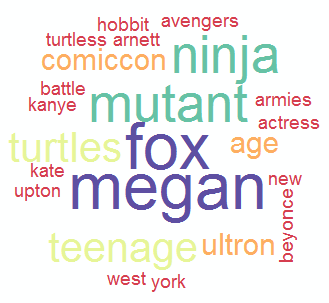
The above word cloud was generated by a computer program using international news headlines on October 6, 2014. This topic was labeled #7: “fox,megan,mutant”.

One powerful and completely automated method for calculating topics from a large volume of data is to use machine learning. Specifically, unsupervised learning in the form of clustering, can clump documents together into cohesive topics. Once clustered, it’s just a matter of finding the most popular terms and we can derive a general sense of topic from each group.

In this article, we’ll explore using clustering for automatically discovering trending topics in a large list of news headlines. We’ll utilize machine learning and unsupervised learning with K-means to automatically relate news headlines by topic, and ultimately derive trending topic keywords from each group.

Machine Learning and News

Machine learning is often better known for its processing of images and sound. However, it’s also highly used in processing text as well. Most types of data can be represented in digital format, and thus, processed using computer algorithms. News stories are already processed on a daily basis by robots. High-frequency traders utilize a variety of computer algorithms to gauge the stock market and take advantage of trends in news. Some of their trigger points include sentiment analysis, breaking stories, and trending topics.

Consumers aren’t the only ones using computer algorithms to process the news, however. Publishers do it too. As long as the published news stories are accurate, most readers probably don’t even notice the difference.

Taking a step back from the publishing of news stories itself, let’s see what a computer program can discover in a large volume of headlines.

The Source of Data

For this article, a large collection of news headlines from the Associated Press Video Hub web site will be used. The web site contains thousands of breaking news stories from around the world. Stories range in topic, depending on popular issues at the time, and remain on the site for a limited duration of time.

Since the time-limit of stories is limited, this gives us a reference window in time to analyze the data set for trending topic information. Otherwise, we might be calculating trending topics over an entire history of news stories (which would hardly be “trending”, and rather, “categorical” instead).

This project takes advantage of direct access to the VideoHub database of stories, extracting over 12,000 news headlines for processing. Let’s see what we can do.

Including Packages

This project uses the R libraries listed below. You’ll want to include these in your project, if you’re following along with the code:

# Set java_
Sys.setenv(JAVA_HOME='C:\\Program Files\\Java\\jre1.8.0_20')

# Install packages if needed.
packages <- c("rJava", "RWeka", "RMongo", "gtools", "openNLP", "tm", "plyr", "RColorBrewer", "wordcloud")
if (length(setdiff(packages, rownames(installed.packages()))) > 0) {
    install.packages(setdiff(packages, rownames(installed.packages())))  
}

library(rJava)
library(RWeka)
require(tm)
require(openNLP)
require(RMongo)
require(plyr)
require(gtools)
require(RColorBrewer)
require(wordcloud)

Reading News Headlines

We’ll start by extracting the news headlines from a Mongo database. We can do this in R using the following code:

# Connect to QA database.
mongo <- mongoDbConnect("news", "news.local.server", 27017)

# Login.
auth <- dbAuthenticate(mongo, "user", "pass")

# Find all published stories.
docs <- dbGetQueryForKeys(mongo, "news", "{isPublished: true, isBreakingNews: true}", "{ storyNumber: 1, title: 1 }", 0, 9999999)

# Disconnect from the database.
dbDisconnect(mongo)

Cleaning Documents

With our data loaded, we’ll want to do a little bit of cleaning up. First, we’ll remove news headlines with empty titles (every database has stuff like this, right?). Next, we’ll extract a list of noun-phrases from each headline. This fosters clustering and helps to avoid grouping of verbs and other potentially less key phrases. In R, we can use the openNLP library to find these terms and append the result as an additional “summary” column in our document table.

# Helper method for breaking a sentence into words by marking words with parts-of-speech tags.
PTA <- Maxent_POS_Tag_Annotator()
tagPOS <- function(x, ...) {
    s <- as.String(x)
    word_token_annotator <- Maxent_Word_Token_Annotator()
    a2 <- Annotation(1L, "sentence", 1L, nchar(s))
    a2 <- annotate(s, word_token_annotator, a2)
    a3 <- annotate(s, PTA, a2)
    a3w <- a3[a3$type == "word"]
    POStags <- unlist(lapply(a3w$features, `[[`, "POS"))
    POStagged <- paste(sprintf("%s/%s", s[a3w], POStags), collapse = " ")
    list(POStagged = POStagged, POStags = POStags)
}

cleanLines <- function(lines) {
    lapply(lines, function(d) {
        result <- ''

        # Strip anything in parenthesis from the docs.
        d <- gsub("\\(.*\\)", "", d)

        # Mark-up text with parts of speech.
        posTags <- tagPOS(d)

        # Split the words by space.
        parts <- strsplit(posTags$POStagged, " ")

        # Concat the nouns, indicated by word/NNP.
        result <- ""
        lapply(unlist(parts), function(p) {
            if (grepl(".+/NNP", p)) {
                result <<- paste(result, gsub("/NNP", "", p), sep = " ")
            }
        })

        # Update result.
        d <- result
    })
}

# Remove empty titles.
docs <- docs[docs$title != '',]

# Clean titles to remove invalid symbols and extract noun phrases.
cleaned <- cleanLines(docs$title)

# Append cleaned column as "summary".
docs$summary <- unlist(cleaned)

Introducing the Term Document Matrix

Each news headline will need to be converted into a digital format, capable of being processed by a machine learning algorithm. One method for doing this is to use a term document matrix.

A term document matrix converts a collection of documents (in this case, news headlines) into a multidimensional array of 1’s and 0’s. First, the unique terms in all of the news headlines (also called a corpus) are collected into a dictionary. Next, each news headline is converted into an array of 1’s and 0’s, where the integer represents whether the current dictionary term exists within the news headline (1) or not (0). The value may also represent the number of times the term appears in the document (this is the method used in the code below). Since we’re looping through the dictionary for every news headline, the length of the array for every headline will be the same length as the number of unique terms. This gives us a consistent matrix of digitized documents to work with.

This type of digitization is common in natural language processing. There are also different ways of building the matrix and setting the values for each term, such as by using term frequency inverse document frequency or TF*IDF to indicate not just whether a term exists in the corpus, but its importance as well.

Building a Corpus

Now that we know we’ll be building a term document matrix, we can start building a corpus and tokenizing the result.

# Build a corpus.
corpus <- Corpus(VectorSource(docs$summary))

# Use bigram features (two words per feature). To use unigrams instead, omit the "tokenize" parameter to TermDocumentMatrix().
bigramTokenizer <- function(x) NGramTokenizer(x, Weka_control(min = 2, max = 2))

# Create a term document matrix (bit array where each vocab term is >= 1 if present in the doc).
tdm <- TermDocumentMatrix(corpus, list(removePunctuation = TRUE, stopwords = TRUE, stemming = TRUE, removeNumbers = TRUE, tokenize = bigramTokenizer))

# Remove sparse terms to save memory and speed.
sparse <- removeSparseTerms(tdm, 0.9997)

# Convert the tdm to a matrix.
data <- as.matrix(sparse)

# Transform the data by sentence, rather than words.
data <- t(data)

# Normalize (optional step).
data <- data / 3

Notice, in the above code we remove punctuation, stopwords, numbers, and stem each term using the porter-stemmer algorithm. We then tokenize the corpus by term-pair.

Unigrams, Bigrams, and N-grams, Oh My!

There are several key steps in the digitization process from the code above. The first important step is choosing the type of tokenization to use. The two most common ways to break up a corpus is by making each term a separate feature to cluster upon (unigram) or by using pairs of terms to cluster upon (bigram).

Unigrams are the most simple and work quite well. However, when dealing with text, unigrams will result in matching up “George Bush” with “George Clooney”, since they both contain the same term “George”. In the case of news headlines, there is a fairly big difference between stories about President George Bush and the actor George Clooney.

Bigrams, on the other hand, resolve the confusion by taking into account pairs of words. In the “George” problem, the bigram phrase “george bush” will be unique from “george clooney”, and each may, in fact, form their own topic. One down-side to bigrams is that they tend to create a larger number of unique clusters with less documents in each one. This is because finding documents that contain the same pairs of words is less likely than finding documents with the same single words. It’s important to take this into account, especially when moving further up the chain in word sets (trigrams and n-grams).

The Problem with N-Grams

The higher the match of N-grams, the more likely it is to result in higher variance and potentially over-fitting the data. In the extreme case, a separate cluster will match each sentence in the set, rendering the clustering effectively useless. In order to group sentences into clusters, matches are required between the N-grams. However, if every sentence is its own N-gram, none will match (unless there is a duplicate news headline).

Considering this, we’ll stick with no larger than bigrams for tokenizing the set of terms.

Stripping Sparse Terms

Simply tokenizing the corpus and running it through an unsupervised clustering algorithm will likely provide some impressive results right at the start. However, for larger data sets (even just 10,000 documents), there may be considerable memory constraints and speed issues when processing with R.

Luckily, we probably don’t need all of the terms in our corpus. Many of the terms are completely unique, only found in the single document themselves. Other terms are only found in just 1 or 2 other documents. These terms can be dropped from clustering to reduce memory usage and processing time. We make a call to removeSparseTerms() to perform this action.

Removing sparse terms can be thought of as a form of compression, in that we’re eliminating less meaningful data points, while still retaining the overall picture of the data. By removing sparse terms from the news headline data set, memory usage was reduced from 2GB down to just 91MB.

K-Means Clustering

Finally, the fun part begins. It’s time to cluster the data and see what we get. Clustering is part of exploratory data analysis, in that it provides a different picture of the data. You can get a view of common elements within the data and begin to see key features that are related amongst the different data points in the set. We can run K-means in R with the following code:

# Run K-means using K clusters (rule of thumb: K = sqrt(n/2)).
cl <- kmeans(data, sqrt(nrow(data) / 2))

# Append the assigned cluster, original title, and summary to each row.
data <- cbind(data, cluster = cl$cluster)
data <- cbind(data, title = docs$title)
data <- cbind(data, summary = docs$summary)

In the above code, we’re automatically choosing the value for K (number of groups) by using a rule-of-thumb calculation of K = sqrt(numberOfDocs / 2).

The kmeans method returns cluster indices in the same order as the data it processed. So, it’s easy to locate the cluster index for each document. We simply step through each document and append the same row from the cluster result. We can also join back in the title and noun-phrase summary on to each row in the data (we had to limit the input to kmeans to just the data we want to cluster on, removing any extraneous data; now we can join that data back in).

Mind the Junk Cluster

When clustering, there is bound to be a cluster that contains more elements than any other cluster. The elements tend to be seemingly unrelated, and in the case of news headlines, they tend to contain few terms or consist mostly of unique noun-phrases. This cluster can be thought of as the “junk cluster”.

The junk cluster consists of documents that were unable to be matched with many others. This can occur if too few features, in the form of matching unique terms, were available. Thus, matches with other documents were either non-existent or limited. The unsupervised learning algorithm tried to do its best by making sense of the data. However, for these documents, the best fit it could find was with other documents that found little or no match.

If the junk cluster is too large, try increasing your feature count by using unigrams, instead of bigrams. Also try increasing the number of clusters (K). Note, if K is increased too far, the result may become less meaningful. The extreme case of this can assign each document to its own cluster, resulting in the same number of clusters as there are documents.

Displaying Word Clouds of Trending Topics

Finally, we can display a visual of each cluster result to get an idea of what the computer program has discovered for trending topics. First, we’ll sort the results by cluster so that everything is together. We’ll then find the most popular terms in each cluster by using a simple word count. Finally, we’ll use the R wordcloud library to display the result.

# Helper method for displaying a word-cloud.
plotGroup <- function(data, groupIndex = 1) {
    # Break up the clusters by group.
    groups <- split(data, data$cluster)

    # Find a target cluster.
    selectedGroup <- lapply(groups, function(g) { if (g[1, 'cluster'] == groupIndex) g })
    # Remove nulls.
    selectedGroup <- selectedGroup[!sapply(selectedGroup, is.null)]

    # Concatenate all of the words in a group into a string.
    words <- ""
    lapply(selectedGroup[[1]]$summary, function(line) {
        words <<- paste(words, line, " ")
    })

    # Draw a word-cloud.
    pal <- brewer.pal(10, "Spectral")
    wordcloud(words, min.freq=1, max.words=30, random.order=FALSE, colors=pal)
}

# Splits the data by group, finds the top term in each group, and appends it to each row (replicating across each row and group).
# The resulting data.frame is a single column with the same number of rows as the original data.frame. Note, to append the top-term column, you need to first sort the original data.frame by group ascending (otherwise they will be out of order).
topTerms <- function(data, column = 'summary') {
    groupTerms <- data.frame()
    groupCount <- length(unique(data$cluster))

    lapply(seq_along(1:groupCount), function(i) {
        s <- data[data$cluster == i, column]
        c <- Corpus(VectorSource(s))
        t <- TermDocumentMatrix(c)
        m <- as.matrix(t)
        v <- sort(rowSums(m), decreasing=TRUE)

        # Take top 3 terms.
        top <- v[1:3]

        # Get the column names, which is the actual term.
        n <- names(top)

        # Concat the list of names into a comma-separated string.
        tag <- paste(n, collapse=',')

        # Replicate the top terms for each row in this group.
        r <- as.data.frame(rep(tag, times=length(s), each=1))

        # Append the row to our result set.
        groupTerms <<- rbind(groupTerms, r)    
    })

    # Set column name for tags.
    colnames(groupTerms) <- c('tags')

    # Return result.
    groupTerms
}

# Sort result by cluster so we can append the tag column. Note, we use a numeric index and not data[,'cluster'] because a term column might actually be "cluster".
sorted <- data[mixedorder(data[,(ncol(data)-2)]),]

# Get the last 3 columns (cluster, title, summary).
sorted <- sorted[,(ncol(sorted)-2):ncol(sorted)]

# Find the top tags in each group.
groupTerms <- topTerms(as.data.frame(sorted))

# Append the tag column to our summary data.
sorted <- cbind(sorted, groupTerms)

# Write result to csv file, sorted by cluster id.
write.csv(sorted, "kmeans.csv")

# Plot a word cloud.
plotGroup(sorted)

Results?

October 6, 2014

78 trending topics from a database of 12,193 international news stories. Examples:

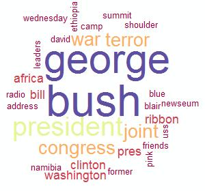
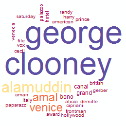
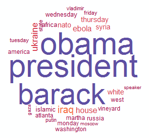
Notice in the above word clouds, George Clooney is a separate cluster from George Bush due to the usage of bigrams. The related topics within those two clusters relate to the actual person, as well. If unigrams were used, it is likely the two clusters would be merged into one.

We can retrieve the entire list of topics to get an overhead view of the result. If we sort by the number of matching stories within each cluster, we can also see which topics were the most popular. The following code will extract the list of topics and their associated story counts (note, the first and largest topic is the junk cluster):

# Get a unique list of trending topics with their frequency count (number of stories classified under each topic).
tags <- count(data$tags)

# Sort the list with the most popular topic first.
tags <- tags[order(tags$freq, decreasing=TRUE),]

Trending Topics

voiced,sound,ukraine,9853
english,voiced,open,654
cup,ryder,europe,112
state,islamic,iraq,109
world,cup,usa,86
new,york,fashion,82
minute,showbiz,asia,80
president,obama,barack,52
champions,league,voiced,51
gaal,van,voiced,49
open,cilic,nishikori,49
bouchard,errani,petkovic,48
world,championships,bwf,48
cup,rogers,voiced,43
bayern,munich,english,39
grand,prix,czech,37
brown,michael,ferguson,35
madrid,atletico,cup,34
louis,cardinals,missouri,32
house,white,secret,30
festival,film,venice,29
clooney,george,alamuddin,28
minister,prime,nouri,28
rice,ray,nfl,28
missouri,ferguson,brown,25
general,assembly,ban,23
new,city,york,23
maria,voiced,english,20
city,manchester,munich,19
president,barack,islamic,19
challenge,pro,usa,18
championship,pga,mcilroy,18
virginia,university,galveston,18
state,john,kerry,17
championship,lpga,park,16
korea,north,afc,16
formula,beijing,english,15
latvala,rally,jari-matti,14
ancelotti,voiced,english,13
city,kansas,royals,13
evergrande,guangzhou,voiced,13
world,championships,english,13
carolina,south,alabama,12
boston,red,sox,11
world,center,trade,11
australia,rally,ogier,10
bush,george,president,10
helen,mirren,hundred-foot,10
china,voiced,english,9
dyche,sean,garry,9
england,voiced,english,9
sotloff,steven,islamic,9
bay,rays,tampa,8
hamas,israel,gaza,8
bank,classic,west,7
control,disease,prevention,7
fox,megan,mutant,7
open,tenerife,boulden,7
plate,river,copa,7
voiced,english,team,7
chloe,grace,moretz,6
michael,sam,cowboyss,6
murray,sound,djokovic,6
abe,assembly,govt,5
beijing,guoan,guizhou,5
central,command,u.s.,5
championships,rowing,world,5
english,germany,voiced,5
holder,attorney,eric,5
korea,north,south,5
missouri,sunday,crowdss,5
stadium,yankee,derek,5
angeles,california,highway,4
angelou,clinton,manhattan,4
chelsea,mourinho,jose,4
continental,cup,europe,4
simeone,voiced,english,4
brown,chief,ferguson,3

Conclusion

The trending topics compiled in this article seem to paint a fairly descriptive picture of the breaking stories of the day. It’s possible to take the clustering method further, by combining multiple days of trending topics together over a longer stretch of time. The resulting topics could, themselves, be clustered to help locate longer-term trends throughout the month. It’s also possible to track increasing and decreasing popularity of the stories over lengths of time.

It’s important to keep in mind that clustering is a form of exploratory analysis. As with any type of exploration of data, results may fluctuate. Clustering uses random initialization points (centroid start locations), which often leads to different results at the end of each process. It can also be difficult to judge the level of success from a clustering result, since the end result is usually not known.

Even with the above subtleties in mind, machine learning can be a powerful method for analyzing data and gaining distinct insight into trends, often hidden to the human eye.

About the Author

This article was written by Kory Becker, software developer and architect, skilled in a range of technologies, including web application development, machine learning, artificial intelligence, and data science.science.

Sponsor Me