An Intelligent Approach to Image Classification By Color

Introduction

Machine learning sounds like a fancy term. Depending on which recent sci-fi film you may have watched, it may even invoke a sense of fear. However, it’s actually a powerful set of algorithms and techniques for allowing a computer program to intelligently arrive at a solution, without explicitly telling it how to do so. Tasks such as recognizing handwritten digits, driving a car, and finding patterns in large amounts of data are examples of where machine learning typically excels over traditional programming techniques.

In a traditional computer program, the programmer writes the code, telling the computer exactly what to do. If A then do B. If C then do D. However, with machine learning the programmer provides certain initial training criteria, such as showing examples of A and C, and allows the computer to arrive at its own decision, based upon what it’s learned. So for example, by watching a steering wheel turn left or right depending on which way the road is curving, a computer can learn how to drive a car.

Red

Green

Blue

In this tutorial, we’ll describe how to classify any image as being red, green, or blue, in overall color. The example program will use a neural network, trained using backpropagation on a subset of example data. The training data will include a few hundred images, which have already been classified as RGB. Once fully trained, the neural network will classify an additional set of images, after which its accuracy may be calculated. In the end, the program will achieve an accuracy of 97.6% on images that it’s never seen before! Not bad.

Can’t This Be Done With a Simple Count of Colors?

Let’s get the easy question out of the way. A non-machine learning approach to classifying an image as red, green, or blue might entail a basic strategy. You could simply count the number of pixels that are red, green, or blue and choose the greatest count as the classification. For example, for each pixel, examine the red, green, and blue channel and pick the channel with the greatest value. For example in RGB, (255, 100, 0) is red; (85, 86, 84) is green, etc. Add up the total for each channel, for every pixel, and classify the image based upon the greatest sum. Training isn’t even required!

Results

So, how does this algorithm fare?

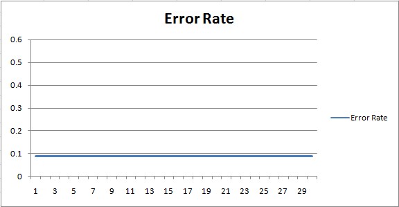
The above chart shows the constant error rate at 0.09 (9%). No learning is achieved with a traditional algorithm. The computer simply follows the explicit instructions to decide the color.

On a training set of 258 images, the algorithm scored an accuracy of 91.02%. On the test set, consisting of 470 images, it scored 93.6%. Not bad. But, with some artificial intelligence, I think we can do better.

Figuring Out What to Teach the Computer

We need to determine some minor calculations before we can start our machine learning implementation. First, we need to consider the data. We’ll be converting hundreds of images into a format that is readable by the computer. This is typically called image recognition / machine vision. The idea is that we’ll convert each image into a comma-separated list of pixel values. Each pixel will have 3 values from 0 to 255 - one value for each color channel (red, green, blue), in that order. Since our csv file could grow extremely large, quite quickly, we’ll restrict the data to 64x64 PNG images. This means we’ll have 12,288 values to process (64 64 3).

Each pixel color value will be an input into our machine learning algorithm. Our output will consist of 3 possible classifications: red, green, or blue. The output will indicate the selected overall color that the computer thinks the image is. With the specifications out of the way, let’s move on to the machine learning part!

Plugging in a Neural Network

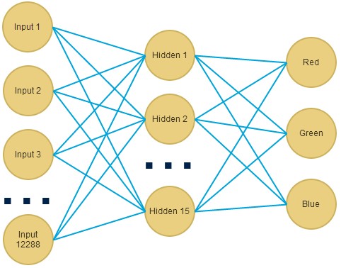
Our first try at implementing machine learning for classifying an image by color in red, green, blue, is to use a neural network. The example program uses NeuronDotNet in C# .NET to implement the neural network. As mentioned above, we’ll use 12,288 inputs, some guess at a number of hidden neurons (we’ll use 15 neurons in 1 hidden layer), and 3 outputs. The setup appears as follows:

BackpropagationNetwork network;

LinearLayer inputLayer = new LinearLayer(12288);
SigmoidLayer hiddenLayer = new SigmoidLayer(15);
SigmoidLayer outputLayer = new SigmoidLayer(3);

BackpropagationConnector connector = new BackpropagationConnector(inputLayer, hiddenLayer);
BackpropagationConnector connector2 = new BackpropagationConnector(hiddenLayer, outputLayer);
network = new BackpropagationNetwork(inputLayer, outputLayer);
network.Initialize();

With the setup complete, it’s time to read our comma-delimited file of pixel values and train the network.

Reading in the Pixel Values

We’ll use the C# .NET CsvHelper class to process the data file to read the pixel values.

using (FileStream f = new FileStream(@"C:\...\colors.csv", FileMode.Open))
{
  using (StreamReader streamReader = new StreamReader(f))
  {
    using (CsvReader csvReader = new CsvReader(streamReader))
    {
      while (csvReader.Read())
      {
        double[] row = new double[12288];
        double label = Double.Parse(csvReader.GetField(12288));

        for (int i = 0; i < 12288; i++)
        {
          double d = (Double.Parse(csvReader.GetField(i)) - (double)127) / (double)255;
          row[i] = d;
        }

        // Format output.
        double[] output = FormatOutputVector(label);

        trainingSet.Add(new TrainingSample(row, output));
      }
    }
  }
}

// Begin training.
network.Learn(trainingSet, 30);

The above code loops through the file and reads each comma-separated pixel value. We don’t actually care about the order of red, green, blue - we’ll leave it to the computer’s intelligence to figure that out. We simply read each value and store it in the input array, for assignment to the trainingSet collection.

Note, we normalize each pixel value so that it falls between -0.5 - 0.5. This allows for easier learning. We use the formula X = (X - avg) / max - min. In our case, we’ll use X = (X - 127) / 255. Alternative methods of feature scaling include X = (X - min) / (max - min) or X = X / 255, which normalizes the value to be between 0 - 1.

Testing the Neural Network Accuracy

After backpropagation training is complete, we load another set of images for the test set. The test set consists of images never before seen by the computer program. This allows us to gauge the neural network’s accuracy on a whole new set of images.

We load the test set using the same code as shown above. We then run the neural network on the each row (image) in the data and score its output.

Results?

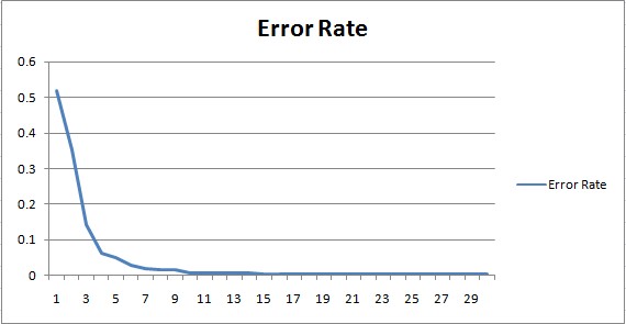
On the training set, the neural network achieves an accuracy of 100%, in just 30 epochs / iterations. This is already 10% better than the non-machine-learning approach. In fact, it’s perfect.

On the test set, the neural network achieves an accuracy of 97.6%. Considering that these are images the program has never seen before, that’s pretty impressive.

Notice in the error rate learning curve, the program quickly achieves a high degree of accuracy on the training set, in just 3 iterations. The remaining iterations fine-tune the accuracy, as the program learns to recognize more details about the images.

Trying it With a Support Vector Machine (SVM)

The neural network worked pretty well. Let’s give it a try with a support vector machine. Unlike a neural network, which classifies using sigmoid activated neurons, a support vector machine classifies by finding a separation line between the data points that minimizes error. In that regard, a neural network may pick up more detailed differences between data points. A support vector machine concerns itself more-so with the greatest differences between the data.

Reading in the Pixel Values for the SVM

We can set up an SVM in C# .NET using the SVM library, which is built upon libsvm. First, we’ll read in the training set, just as we did in the above example. The code appears, as follows:

Problem train = GetProblemSet(@"C:\...\colors.csv");
Problem test = GetProblemSet(@"C:\...\colorstest.csv");

private static Problem GetProblemSet(string pathName)
{
  // Process the list of indices as input into an SVM.
  List<double> vy = new List<double>();
  List<node[]> vx = new List<node[]>();
    
  using (FileStream f = new FileStream(pathName, FileMode.Open))
  {
    using (StreamReader streamReader = new StreamReader(f))
    {
      using (CsvReader csvReader = new CsvReader(streamReader))
      {                       
        while (csvReader.Read())
        {
          double[] row = new double[12288];
          double label = Double.Parse(csvReader.GetField(12288));

          for (int i = 0; i < 12288; i++)
          {
            double d = (Double.Parse(csvReader.GetField(i)) - (double)127) / (double)255;
            row[i] = d;
          }

          vy.Add(label);

          Node[] x = new Node[row.Length];
          for (int i = 0; i < row.Length; i++)
          {
            x[i] = new Node(i, row[i]);
          }

          vx.Add(x);
        }
      }
    }
  }

  return new Problem(vy.Count, vy.ToArray(), vx.ToArray(), vx[0].Length);
}

Notice, we’re once again normalizing the input values with the same formula, to force the input values to fall between 0-1. We’re also using the CsvHelper C# .NET class to parse the comma-separated file. The only real difference is the population of the “Problem” object, which is required by the SVM class. It’s really just a collection of doubles for input (vx), output (vy), and lengths.

Initializing the SVM

Parameter parameters = new Parameter();

// These magic numbers must be guessed or calculated by iterating over various values.
double C = 2048, gamma = 0.0001220703125;

// Find optimal C and Gamma values.
ParameterSelection.Grid(train, parameters, "params.txt", out C, out gamma);
parameters.C = C;
parameters.Gamma = gamma;
parameters.KernelType = KernelType.RBF;

Model model = Training.Train(train, parameters);

As you can see in the above code, the key behind an SVM are the values selected for C and gamma. These values determine how the separation line is drawn within the data, and thus, how well the SVM will perform on the training data. To arrive at the best values, we run a ParameterSelection method, which iterates over various values to try and find the lowest error rate.

Once we’ve found the estimated optimal C and Gamma values, we can run the SVM on the test data and allow it to predict the result.

double result = Prediction.Predict(model, training);

Results?

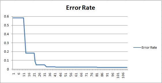
On the training set, the SVM achieves an accuracy of 95.3%. This is already 4% better than the non-machine-learning approach.

On the test set, the SVM achieves an accuracy of 87.6%, which is not quite as good. This is an example of high variance, which usually results from over-fitting to the training set.

Fixing High Variance in an SVM

Since we’re using an SVM, a good way to solve high variance is to simply change the C and Gamma values, which correspond to the learning rate and smoothness, respectively. For high variance, we can try decreasing C and increasing Gamma. Our automated optimization method chose C as 2048. We can tweak it from here.

Lowering C to 1048, and increasing Gamma, results in Training: 100%, Test: 91.5%.
Lowering C to 900, and increasing Gamma, results in Training: 100%, Test: 94.2%.

At this point, the SVM beats the non-machine learning algorithm. Neat!

Another good way to fight high variance is to simply get more data. In this case, that would mean collecting more images. Yet, another option is to reduce the number of features. Since our features represent pixel color values (recall, we have 12,288 of them), that would mean reducing the size of our images. A reasonable action might be to try 32x32 pixel images. That would reduce our feature size to 3,072, a 75% reduction in features.

Try It Yourself

Demo ColorBot

As a final piece of the experiment, the neural network has been enhanced as a web application and is available online. You can watch it attempt to classify images by color, selecting images at random from the test set, or upload your own.

The web application is written in node.js, and uses the brain neural network library. The neural network itself, was pre-calculated and hard-coded into the web application as JSON. The test set image data is stored via MongoDb.

By the way, if you enjoyed this article, you might also like my experiments with self-programming artificial intelligence and genetic algorithms.

Download @ GitHub

Source code for ColorBot (the node.js version of the neural network) is available on GitHub.

About the Author

This article was written by Kory Becker, software developer and architect, skilled in a range of technologies, including web application development, machine learning, artificial intelligence, and data science.

Sponsor Me

• ai
• artificial intelligence
• big data
• high variance
• machine learning
• ml
• neural network
• support vector machine
• svm

Share